A Python program can recover a known timing shift, reproduce its saved output, and still lack the evidence needed to explain a star’s orbit. Eclipse Atlas reached that boundary in its second phase.
The first research note described a pipeline for measuring eclipsing binaries in public TESS observations and reassessing published companion candidates. The next phase tested whether the measurement uncertainties, long-term trends, and proposed independent checks could support the intended interpretation.
The strongest retained result is a scoped calibration of individual eclipse-time intervals. The complete long-term drift procedure did not pass scientific acceptance. A general eclipse-shape test and the planned archival-photometry route also stopped under their predefined rules. The analysis line is now closed, with its software, conditional results, and failed tests preserved for review.
There is no independently confirmed new companion or reliable excess apsidal motion from this project. The later validation does not establish that the published candidates are false, either.
Three claims that require separate tests
An eclipsing binary produces two recurring dips as its stars pass in front of each other. A timing program fits the center of each dip and compares it with a calculated schedule. This difference is the O−C residual: observed minus calculated.
The primary and secondary eclipses provide related measurements. Changes shared by both can have different causes from changes in their relative timing. Apsidal motion, the gradual rotation of an eccentric orbit, is one possible source of a differential trend. Changes in brightness distribution and errors in the measurement procedure can also affect that trend.
The second phase separated three questions:
- Does an interval around one measured eclipse time contain its defined reference time at the expected frequency?
- Does the procedure for combining observations and fitting a trend have the expected false-alarm behavior?
- Can the inferred trend be assigned to orbital physics and compared reliably with stellar contributions?
Each step depends on additional assumptions. Calibrating the first measurement does not validate the complete chain.
| Component | Result retained | Boundary of the claim |
|---|---|---|
| Individual eclipse-time intervals | Passed the specified development evaluation | Restricted data product, sampling, selection, and definition of time |
| Long-term differential trends | Conditional node-model simulations and diagnostic results | Full-pipeline calibration and transfer from the node simulator remain unestablished |
| Extra eclipse-shape information | Measurable cases and documented blind spots | General feasibility rule returned STOP |
| Archival-photometry test | Reconstructed joint predictions and a failed prediction gate | No new archive light curves were downloaded or measured |
Calibrating the quantity the program actually measures
A fitted eclipse center depends on the estimator. A template’s center, another model’s fitted center, and the instant of geometric conjunction need not coincide exactly. Before checking uncertainty, the reference answer has to match the quantity being measured.
The retained calibration used TESS SPOC observations with 120-second exposures and SAP flux, which is the simple-aperture photometry product. Periodic-variability subtraction, or prewhitening, was disabled; the sample had predefined variability and contamination cuts and required usable space for injections. The synthetic reference used a noiseless twin evaluated with the matched estimator.
Coverage then asks a concrete question: across repeated evaluations, how often does the reported interval contain that reference? An interval labeled 95% should contain it about 95% of the time under the tested conditions.
| Evaluation | Coverage of nominal 95% interval | Coverage of nominal 68% interval |
|---|---|---|
| Synthetic evaluation | 95.1% | 75.4% |
| Injections into real light curves | 96.6% | 77.4% |
The real-light-curve result uses four systems and eight system–sector clusters. Repeated injected events do not create additional independent stars. The coverage analysis accounted for clustering, and the figure reports cluster-bootstrap intervals.
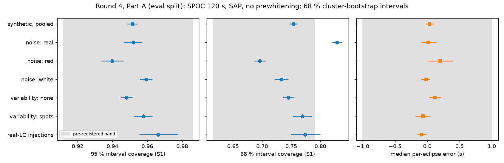
Figure 1. Retained single-eclipse calibration evidence. Horizontal bars are 68% cluster-bootstrap intervals. Gray bands show the preregistered pooled acceptance ranges; noise strata also had separate predefined lower limits. The nominal 68% intervals are conservative. This figure does not validate long-term drift inference. Open full-size figure.
The 68% intervals contain the reference more often than their label suggests. Passing the development rule therefore should not be described as exact Gaussian calibration.
There are further limits. Injecting a template into real residual noise checks how that measurement behaves under the sampled noise. It cannot cover every mismatch between the template and an actual eclipse. Agreement with an estimator-defined reference also cannot establish absolute accuracy relative to geometric conjunction.
The evaluation systems had appeared in earlier development diagnostics. Freezing the evaluation rules provided useful discipline, but it did not turn those systems into a new independent confirmation sample.
A node simulator cannot stand in for the complete pipeline
The trend analysis summarizes observations into sector-level timing nodes. It then fits a differential trend while allowing additional independent variation between sectors.
A simulator that starts with those nodes can test the statistical model efficiently. The complete pipeline has more stages: light-curve preparation, event fitting, quality cuts, node construction, uncertainty treatment, and trend estimation. Those stages can change the distribution reaching the final fit.
The transfer study compared the two layers and examined differences in node counts, sampling layouts, uncertainty floors, and simulated activity. After matching composition, the 95% interval for one pipeline-minus-node false-alarm-rate difference was −0.002 to 0.062.
That interval includes zero. A remaining discrepancy was not established, and the uncertainty was also too wide to establish useful transfer accuracy. The earlier independent confirmation benchmark had failed. Node-level support could not replace either missing validation.
This resembles testing a downstream estimator on a prepared dataset and then placing it behind an ingestion and transformation pipeline. The downstream test is informative only to the extent that the delivered inputs satisfy its assumptions. Here, those assumptions include dependence between observations, so matching file formats and array dimensions is insufficient.
Slowly changing errors can resemble a trend
Independent jitter allows observations to scatter separately. An omitted error that changes gradually across observing seasons can instead create a smooth pattern that a trend fit treats as evidence.
The project tested this risk with synthetic differential timing nodes, varying correlation timescale, amplitude, and sampling layout. No such process was measured in an actual target by these experiments.
One saved condition illustrates the size of the risk: twelve nodes in four seasons, a 20-second correlated-process amplitude, a 1,000-day correlation timescale, and 10-second independent Gaussian jitter. Among 400 simulated zero-drift cases, 149 were flagged: about 37%, against a nominal 5% threshold. The stated node error was 5 seconds. This is one defined stress-test condition, not a false-positive estimate for the TESS archive.
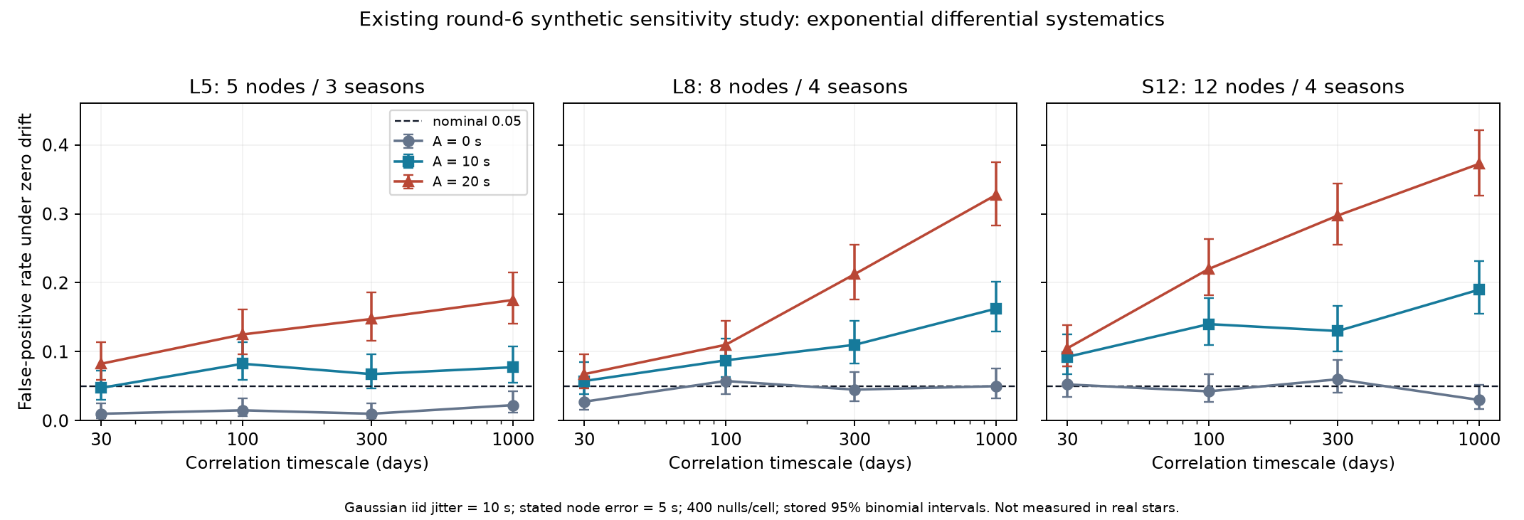
Figure 2. Previously saved simulations, replotted for the review packet. The three panels show fixed layouts; curves vary the synthetic correlated amplitude. The dashed line is the nominal 0.05 rate, and error bars are saved 95% binomial intervals. All plotted conditions use 10-second independent Gaussian jitter. These curves are not measurements of real stellar systematics. No new simulations were run to make this figure. Open full-size figure.
The available diagnostics did not adequately bound this risk. A process that changes little within one observing sector can evade a within-sector scatter check. Different reductions of the same photons can reveal processing differences, but their agreement supplies limited independence against an astrophysical change shared by those photons.
The permitted interpretation remains a descriptive fitted trend, with an interval conditional on the stated noise model. The project has not established that such a trend measures physical apsidal motion.
Eclipse shape supplied useful cases and important blind spots
A brightness distortion can shift the fitted center of an eclipse. Shape information might identify that distortion and help distinguish it from a change in orbital timing.
The difficulty is identifiability. For a small displacement, f(t − δt) ≈ f(t) − δt f′(t). A distortion resembling the local derivative can look like a time shift. Allowing both possibilities in the fit can greatly increase timing uncertainty.
In an idealized full-coverage calculation with white noise and a perfect template, freeing the tested shape parameters increased timing uncertainty by a factor of 11–14. The subsequent simulations used real residual noise and observational coverage to assess detectability under less idealized conditions.
Five reference conditions were selected by timing precision within the development sample. The tested families included unequal eclipse wings, localized bumps, an in-eclipse tilt, and background changes. They were phenomenological distortions, not physical starspot models or measurements of actual shape changes.
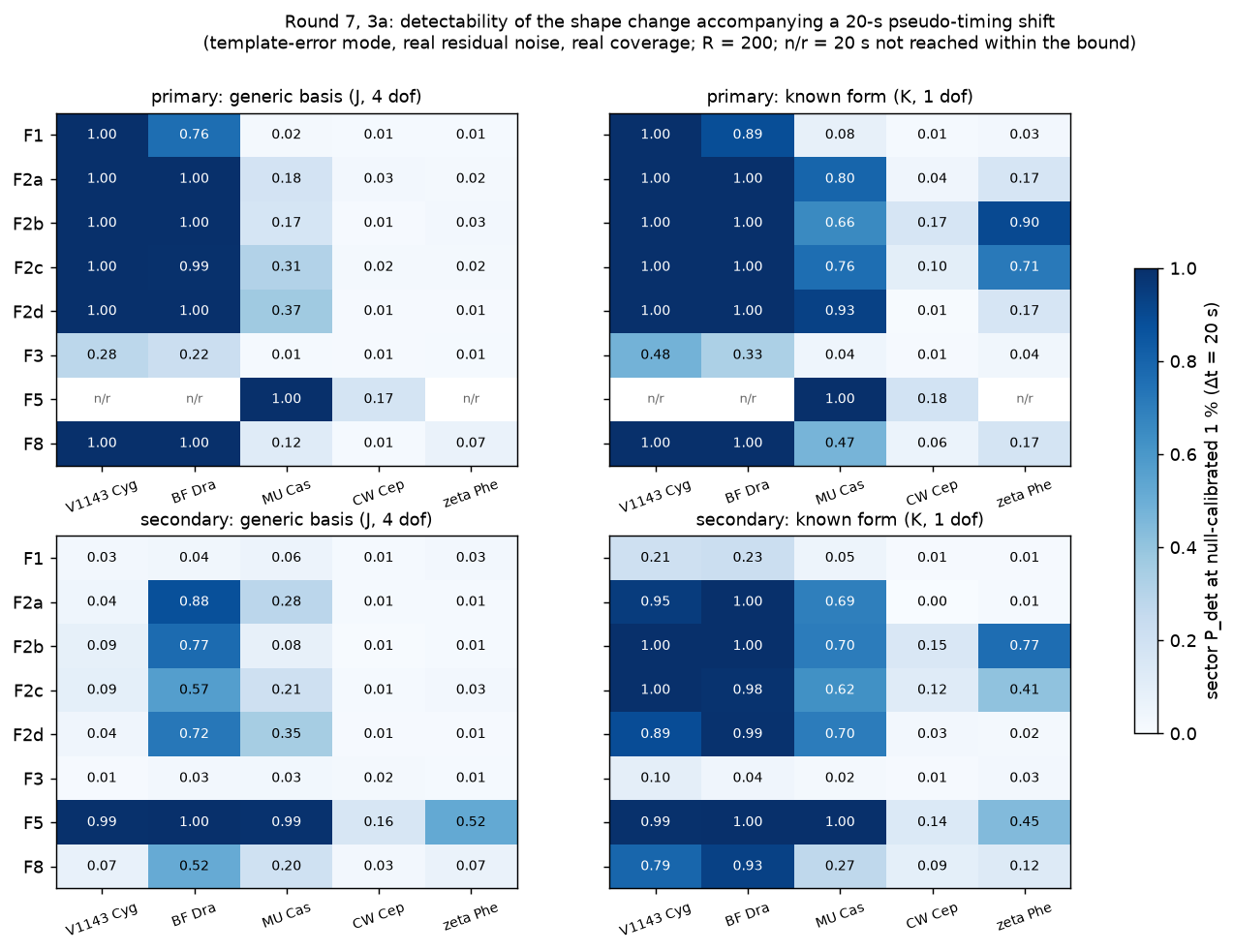
Figure 3. Top: primary eclipses; bottom: secondary eclipses. Left: a generic shape basis; right: the exact distortion form is assumed known. F1 denotes wing asymmetry, F2a–d localized bumps, F3 an in-eclipse tilt, F5 a cubic background, and F8 a combination. The target apparent shift is 20 seconds; n/r means it was not reached within the allowed distortion bound. The displayed 1% threshold is nominal: threshold calibration and distortion evaluation shared noise and did not establish an independent false-flag rate. The five conditions are not a population sample. Open full-size figure.
Some precisely timed primary eclipses revealed injected distortions. Secondary eclipses retained important blind spots, including in the brighter reference conditions. A differential inference needs both eclipse kinds.
Under the predefined rule, only one of five conditions had two measurable distortion families; at least three were required. The outcome remained STOP. Failure to detect a shape change could not exclude a spurious timing shift under these conditions.
This result leaves target-specific physical modeling open. It does not establish that eclipse shape is generally uninformative or that other observations cannot help.
The archival test stopped before acquiring observations
The first article discussed using older observations to distinguish competing forecasts. The later work checked whether those forecasts remained sufficiently informative before downloading archival light curves.
An earlier forecast had sampled geometry and stellar contributions independently and omitted adopted geometry uncertainty floors. The revised calculation reconstructed their joint draws and applied the floors. Preserving those dependencies changed the prediction widths. The upstream adequacy of the geometry models remained a separate limitation.
The proposed comparison used the interval between primary and secondary eclipses at a historical epoch. H_T used the published apsidal-motion rate; H_S used the stellar-contribution prediction. Both were conditional models, and together they did not exhaust the possible physical explanations.
The gate required at least 80% probability of obtaining a Bayes factor of 20 or greater for the generating model in both directions, under every predefined stress variant. To pass, a target had to tolerate a measurement error of at least 600 seconds while meeting those requirements. The measurement-error grid ran from 60 to 10,800 seconds, with an assumed 180-second systematic contribution for the cited example.
One variant, R10, multiplied the published rate uncertainty by ten. It was a literature-motivated sensitivity test. It did not measure tenfold error underestimation in the tested targets.
| Target | Strong support for H_T when H_T generates the data | Strong support for H_S when H_S generates the data |
|---|---|---|
| TIC 253270207 | 77.45% | 0% |
| TIC 146204045 | 87.10% | 5.15% |
These are predicted probabilities under R10 at an assumed 60-second measurement error and the stated historical-epoch setup. They are not significances from observations.
The asymmetric power matters. A failed two-direction gate does not imply zero information. An earlier summary field containing zero meant that no tested precision passed the entire gate; the closeout corrected wording that had interpreted it as zero power at every precision.
The failed gate remained failed after that correction. No target met every requirement. No archive target-coverage query, new observational-product download, or sparse-data timing estimator followed. Consequently, this trial did not measure the actual information in those archives. A redesigned observable or new independent observations would require a separately specified study.
Preserving a result includes preserving its limits
The numerical audit also found a misleading uncertainty field. For the model labeled M5 with three nodes, the posterior standard deviation does not exist. An older finite scale value came from numerical truncation. The software preserves it for historical reproduction while exposing sd_exists, scale_definition, and halfwidth68; the old value must not be reused as a valid standard deviation.
That distinction is easy to miss in a data pipeline. A finite serialized number can pass schema and unit checks while failing to represent the quantity its field name suggests.
The closeout preserved code history, inputs that were excluded from Git, outputs, manifests, and restoration instructions. Restoration checked 2,488 files against their hashes. A separate, limited regeneration check reproduced ten of eleven recorded outputs byte for byte; the remaining difference was cost metadata. The final handover did not rerun the complete scientific workflow.
The backup was on the same physical disk and had no off-disk copy at handover. It protects against some directory-level mistakes, while a disk failure remains a separate risk. This website publishes selected project figures and an evidence appendix; it does not distribute the private backup, raw observations, or third-party paper files.
Existing work narrows the scientific claim
Several general ideas in this phase already have published precedents:
- Carter and Winn (2009) tested timing estimation and uncertainty under correlated noise using simulated transit light curves. The need to calibrate errors under correlated noise is established prior work.
- Mikulášek (2015) developed phenomenological eclipse models for practical light-curve and timing tasks. Template-based measurement and joint use of phase information have a substantial history.
- Liang, Winn, and Albrecht (2022) combined TESS and earlier observations to study starspots, gravity darkening, and stellar orientations in DI Herculis. Their target-specific work is distinct from this project’s limited generic shape budget.
- Jiang’s 2026 preprint examines target-specific stellar effects and sector-level timing in CH Ind and SW CMa. The review packet identifies overlap with the sector-node and stellar-budget approach used here.
The handover’s literature review was bounded and incomplete. Some papers were checked in selected sections; other full texts or citation searches remained unavailable. It did not establish novelty, general superiority, or publication readiness.
The material retained for possible specialist review is narrower: interval coverage under stated TESS conditions, the transfer checks between statistical layers, sensitivity to correlated differential errors, and a quantitative shape-information budget. No external expert has endorsed these as a publishable contribution.
The archived record keeps each result attached to its data conditions, estimator, assumptions, and failed acceptance tests. Any future study would need to identify the missing evidence it can obtain and define its success criteria before reopening that question.
Phase-two research note, published October 14, 2026, Pacific time. The source review packet is dated October 15 UTC and refers to research snapshot research-closeout-v1 (87f8c7d). All three figures are unchanged copies of project outputs supplied with that packet. The phase-two evidence appendix records source documents, scripts, commits, input conditions, figure hashes, and the interpretation corrections. These project results have not been peer reviewed. Preparing this article added no scientific experiments or observational downloads.